In this post I read in a data set in R containing data on used car sale postings on German ebay. The data has been shared on kaggle and can be found here: https://www.kaggle.com/orgesleka/used-cars-database/data

# read in the data
data_df = read.csv("autos.csv",header=TRUE,sep = ",")
# print a summary
summary(data_df)

##               dateCrawled                      name               seller      
##  2016-03-08 15:50:29:     5   Ford_Fiesta        :   336   gewerblich:     2  
##  2016-03-20 16:50:22:     5   Volkswagen_Golf_1.4:   335   privat    :189347  
##  2016-03-26 10:51:07:     5   BMW_318i           :   334                      
##  2016-03-31 17:57:07:     5   Opel_Corsa         :   316                      
##  2016-04-02 14:50:21:     5   BMW_316i           :   258                      
##  2016-03-05 15:48:41:     4   BMW_320i           :   256                      
##  (Other)            :189320   (Other)            :187514                      
##    offerType          price              abtest          vehicleType   
##  Angebot:189341   Min.   :       0   control:91131   limousine :48701  
##  Gesuch :     8   1st Qu.:    1150   test   :98218   kleinwagen:40759  
##                   Median :    2950                   kombi     :34498  
##                   Mean   :   10895                             :19437  
##                   3rd Qu.:    7200                   bus       :15532  
##                   Max.   :99999999                   cabrio    :11668  
##                                                      (Other)   :18754  
##  yearOfRegistration      gearbox          powerPS            model       
##  Min.   :1000                : 10395   Min.   :    0.0   golf   : 15286  
##  1st Qu.:1999       automatik: 39220   1st Qu.:   70.0   andere : 13453  
##  Median :2003       manuell  :139734   Median :  105.0   3er    : 10528  
##  Mean   :2005                          Mean   :  114.7          : 10398  
##  3rd Qu.:2008                          3rd Qu.:  150.0   polo   :  6714  
##  Max.   :9999                          Max.   :19208.0   corsa  :  6415  
##                                                          (Other):126555  
##    kilometer      monthOfRegistration    fuelType                brand      
##  Min.   :  5000   Min.   : 0.000      benzin :114106   volkswagen   :40687  
##  1st Qu.:125000   1st Qu.: 3.000      diesel : 54968   bmw          :20545  
##  Median :150000   Median : 6.000             : 16936   opel         :20427  
##  Mean   :125640   Mean   : 5.733      lpg    :  2732   mercedes_benz:17931  
##  3rd Qu.:150000   3rd Qu.: 9.000      cng    :   308   audi         :16676  
##  Max.   :150000   Max.   :12.000      hybrid :   142   ford         :13093  
##                                       (Other):   157   (Other)      :59990  
##  notRepairedDamage              dateCreated      nrOfPictures   postalCode   
##      : 36542       2016-04-03 00:00:00:  7392   Min.   :0     Min.   : 1067  
##  ja  : 18410       2016-04-04 00:00:00:  7185   1st Qu.:0     1st Qu.:30559  
##  nein:134397       2016-03-20 00:00:00:  6860   Median :0     Median :49661  
##                    2016-03-12 00:00:00:  6853   Mean   :0     Mean   :50892  
##                    2016-03-21 00:00:00:  6843   3rd Qu.:0     3rd Qu.:71577  
##                    2016-03-14 00:00:00:  6691   Max.   :0     Max.   :99998  
##                    (Other)            :147525                                
##                 lastSeen     
##  2016-04-07 00:46:04:    14  
##  2016-04-06 04:17:47:    12  
##  2016-04-06 05:44:34:    12  
##  2016-04-06 08:15:55:    12  
##  2016-04-06 09:46:11:    12  
##  2016-04-06 09:46:51:    12  
##  (Other)            :189275

The data has been accessed by applying web scraping and the data set contains a considerable amount of entries. This also becomes clear from above summary.

I proceed by cleaning the data. Cleaning at this stage consists of filtering out entries with missing data. Since there are many variables the relative share of entries with at least one missing data point is relatively high. Therefore, I reduce the data set to comprise relevant variables only. For this “compact” data set I conduct a cleaning run, in which I remove all entries that have at least one empty data point in them.

– name

– seller

– price

– vehicleType

– yearOfRegistration

– gearbox

– powerPS

– model

– kilometer

– fuelType

– monthOfRegistration

– brand

– postalCode

library(dplyr)
library(magrittr)
data_df = data_df %>% select(name,seller,price,vehicleType,yearOfRegistration,gearbox,powerPS,model,kilometer,fuelType,monthOfRegistration,brand,postalCode)

# filter out empty entries; not using dplyr
for(i in 1:ncol(data_df)){
  data_df = data_df[data_df[,1]!="",]
}

# create a first column plot with mean prices by kilometer group
library(ggplot2)
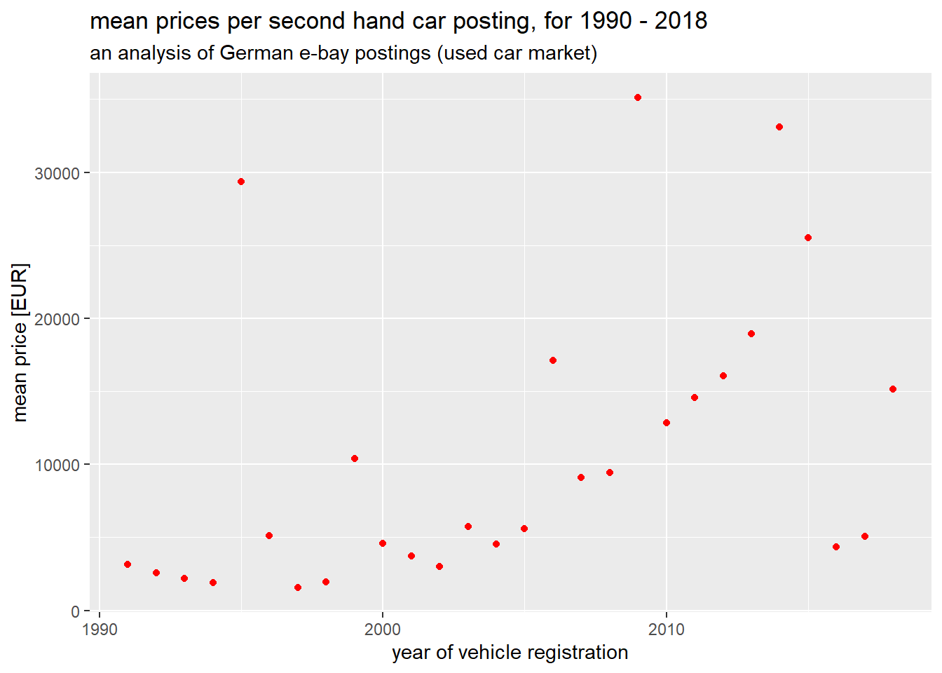
ggplot(summarise(group_by(filter(data_df,yearOfRegistration>1990 & yearOfRegistration<2019),yearOfRegistration),mean=mean(price))) + geom_point(mapping=aes(x=yearOfRegistration,y=mean),color="red") + labs(title="mean prices per second hand car posting, for 1990 - 2018",
                                                                                                                                                                                                 subtitle="an analysis of German e-bay postings (used car market)") + 
  xlab("year of vehicle registration") + 
  ylab("mean price [EUR]")

In following posts I will explore this data set further. I will use the data set further to explore used car market in Germany. Also, I will clean the data much more and look for outliers in the data set.

Linnart Felkl

Data scientist focusing on simulation, optimization and modeling in R, SQL, VBA and Python