In a previous post I showed how a single warehouse location problem can be approached by locating the warehouse near its center of mass. In this post we want to locate multiple warehouses at their center of mass.

We will use the functions already defined in previous posts.

In http://www.supplychaindataanalytics.com/single-warehouse-problem-locating-warehouse-at-center-of-mass-using-r/ I provided a function for locating a single warehouse at its center of mass.

In http://www.supplychaindataanalytics.com/proximity-based-spatial-customer-grouping-in-r I showed how to group customers based on spatial proximity clustering.

# example see here: http://www.supplychaindataanalytics.com/single-warehouse-problem-locating-warehouse-at-center-of-mass-using-r/
center_of_mass <- function(x,y,w){
  c(crossprod(x,w)/sum(w),crossprod(y,w)/sum(w))
}

# example see here: http://www.supplychaindataanalytics.com/proximity-based-spatial-customer-grouping-in-r
initial_centers <- function(customers,centers){
  quantiles <- c()
  for(i in 1:centers){
    quantiles <- c(quantiles,i*as.integer(nrow(customers)/centers))
  }
  quantiles
}

We will combine these two approaches to solve a multiple warehouse location problem using center of mass theory. This approach is applicable when we already know how many warehouses we want to operate. The approach in the post at hand will not suffice to solve a problem in which we do not know yet how many warehouses we actually want to operate.

I start by creating a dataframe with 1000 randomly distributed customers with randomly distributed demand

customer_df <- as.data.frame(matrix(nrow=1000,ncol=3))
colnames(customer_df) <- c("lat","long","demand")
customer_df$lat <- runif(n=1000,min=-90,max=90)
customer_df$long <- runif(n=1000,min=-180,max=180)
customer_df$demand <- runif(n=1000,min=0,max=10)
head(customer_df)

##         lat       long   demand
## 1 -42.50378  137.62188 9.608067
## 2  47.79308  101.30536 9.510299
## 3 -14.17326   24.38595 1.610305
## 4 -85.34352 -151.29061 6.394425
## 5 -26.31244  112.75030 6.972434
## 6  55.01428   58.17198 2.797564

Next, I group the customers using the approach shown in a previous post and applying the defined function initial_centers. I want to locate 20 warehouses so I group customers into 20 groups.

centeroids <- initial_centers(customer_df[,-3],20)
cluster_obj <- kmeans(customer_df[,-3],centers = customer_df[centeroids,-3])
customer_df$group <- cluster_obj$cluster
head(customer_df)

##         lat       long   demand group
## 1 -42.50378  137.62188 9.608067     2
## 2  47.79308  101.30536 9.510299     4
## 3 -14.17326   24.38595 1.610305     6
## 4 -85.34352 -151.29061 6.394425     8
## 5 -26.31244  112.75030 6.972434    18
## 6  55.01428   58.17198 2.797564    16

As displayed above I added the clustering-based group index to the customer dataframe.

Now, I will define a function that will loop through every customer group and identify the center of mass. The requirement is that a dataframe must be inputted, containing a latitude, longitude, demand and group column – in exactly this format:

multiple_centers_of_mass <- function(df){
  result_df <- as.data.frame(matrix(nrow=nrow(df),ncol=6))
  colnames(result_df) <- c("lat","long","demand","group","com_lat","com_long")
  result_df[,c(1,2,3,4)] <- df
  for(i in 1:length(unique(df[,4]))){
    sub_df <- result_df[result_df$group==i,]
    com <- center_of_mass(sub_df$lat,sub_df$long,sub_df$demand)
    result_df$com_lat[result_df$group==i] <- com[1]
    result_df$com_long[result_df$group==i] <- com[2]
  }
  result_df
}

Let us test the multiple_centers_of_mass functio that I just defined:

com_df <- multiple_centers_of_mass(customer_df)
head(com_df)

##         lat       long   demand group   com_lat   com_long
## 1 -42.50378  137.62188 9.608067     2 -25.97973  158.17382
## 2  47.79308  101.30536 9.510299     4  63.58158   84.91329
## 3 -14.17326   24.38595 1.610305     6 -21.20417   26.80993
## 4 -85.34352 -151.29061 6.394425     8 -64.12072 -145.48419
## 5 -26.31244  112.75030 6.972434    18 -33.15564   99.15738
## 6  55.01428   58.17198 2.797564    16  35.04988   44.42388

Lets visualize the test results using a scatterplot from the ggplot2 R package. Below you see the warehouse locations (centers of mass):

library(ggplot2)

lat_wh_vc <- unique(com_df$com_lat)
long_wh_vc <- unique(com_df$com_long)
warehouse_df <- as.data.frame(matrix(nrow=length(lat_wh_vc),ncol=2))
warehouse_df[,1] <- lat_wh_vc
warehouse_df[,2] <- long_wh_vc
colnames(warehouse_df) <- c("lat","long")
ggplot(warehouse_df) + geom_point(mapping = aes(x=lat,y=long)) + xlim(-90,90) + ylim(-180,180)

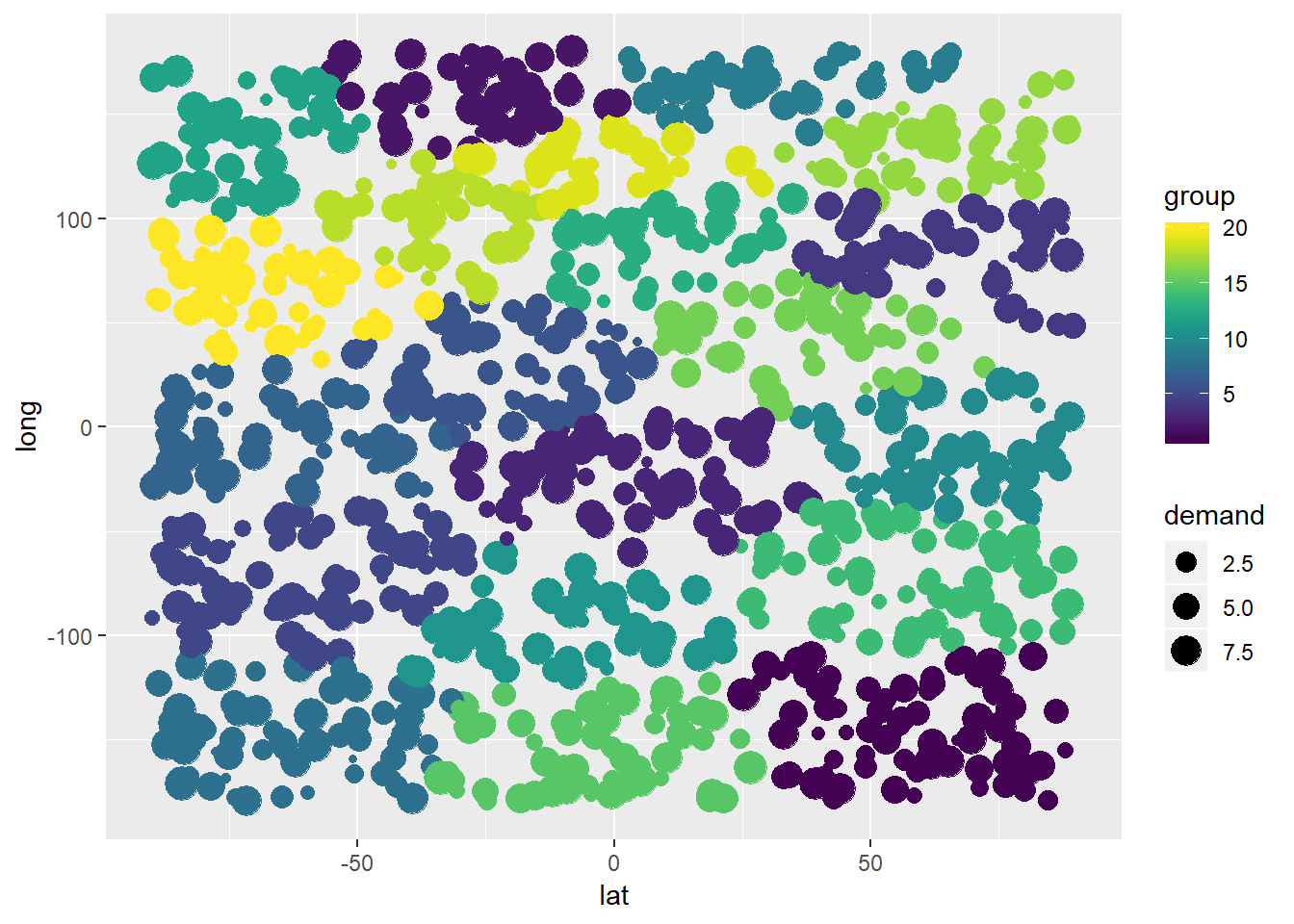
The customers are grouped as shown below:

library(viridis)

## Warning: package 'viridis' was built under R version 3.5.3

## Loading required package: viridisLite

ggplot(com_df) + geom_point(mapping = aes(x=lat,y=long,color=group,size=demand)) +
  xlim(-90,90) + ylim(-180,180) + scale_color_viridis(discrete = FALSE, option = "D") + scale_fill_viridis(discrete = FALSE) 

Linnart Felkl

Data scientist focusing on simulation, optimization and modeling in R, SQL, VBA and Python