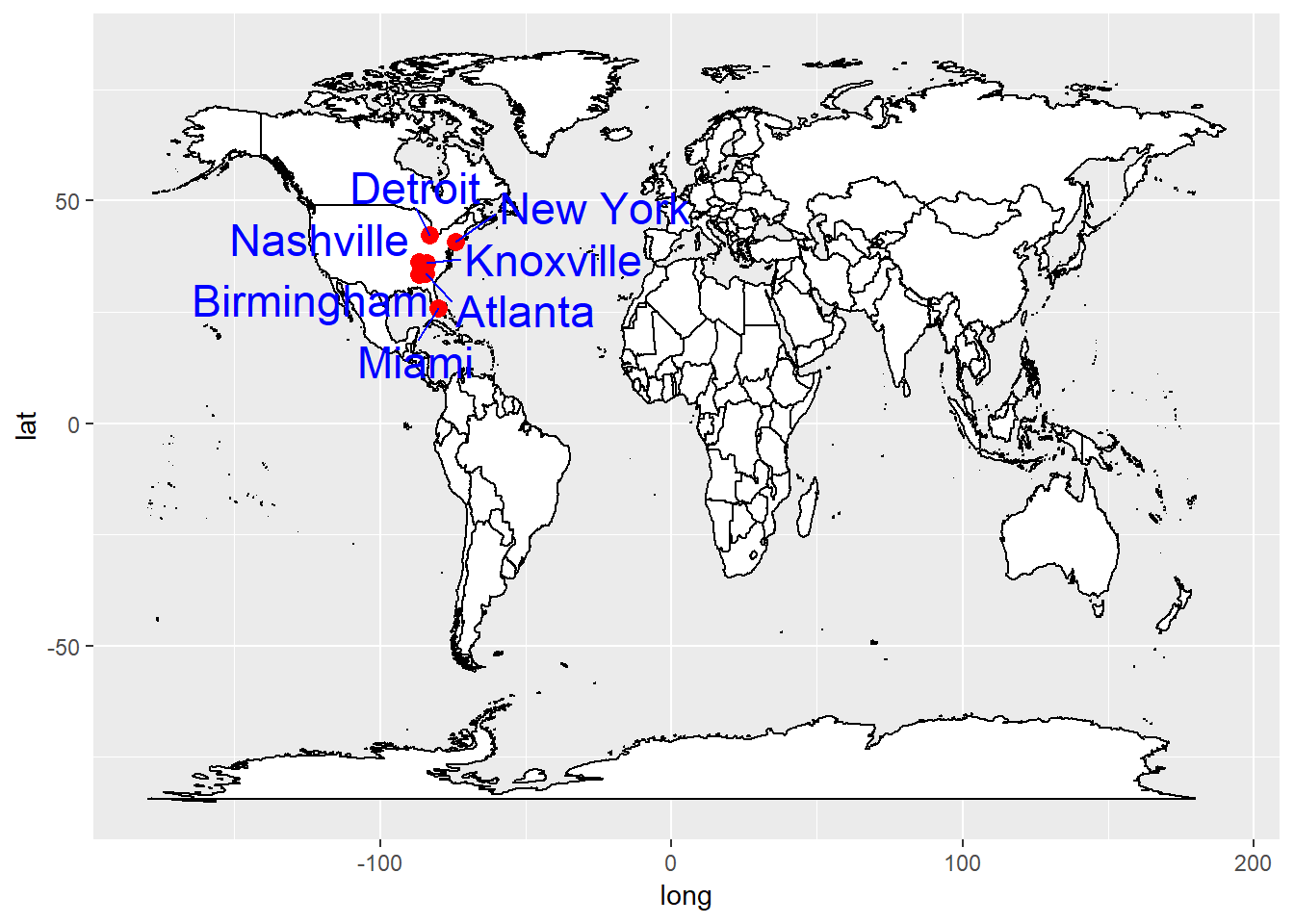
In this post I want to demonstrate how spatial locations can be plotted onto map tiles using the ggplot2 package in R.

For this, we first load the relevant packages. In addition, we define a geocoding function using the Open Street Map API. The geocoding function was obtained from https://datascienceplus.com/osm-nominatim-with-r-getting-locations-geo-coordinates-by-its-address/.

In the next step, using the map_data function from the ggplot2 package, we collect a map in form of a dataframe suitable for plotting. We then also create a list of city names manually, and convert these city names into coordinates using the geocoding function.

Using the ggplot2 and ggplot2 the geocoded data points are then visualized on a world map.

# import relevant libraries 
library(ggplot2)
library(ggrepel)

# osm geocoder
osm_geocoder <- function(address = NULL)
{
  if(suppressWarnings(is.null(address)))
    return(data.frame())
  
  tryCatch(
    d <- jsonlite::fromJSON( 
      gsub('\\@addr\\@', gsub('\\s+', '\\%20', address), 
           'http://nominatim.openstreetmap.org/search/@addr@?format=json&addressdetails=0&limit=1')
    ), error = function(c) return(data.frame())
  )
  
  if(length(d) == 0) 
    return(data.frame())
  
  return(data.frame(lon = as.numeric(d$lon), lat = as.numeric(d$lat)))
}

# core part 
# data preparation
world <- map_data("world")

points_df <- data.frame(matrix(nrow=0,ncol=2))
colnames(points_df) <- c("long","lat")
city_list <- c("New York City, New York, USA",
               "Detroit, Michigan, USA",
               "Atlanta, Georgia, USA",
               "Birmingham, Alabama, USA",
               "Miami, Florida, USA",
               "Nashville, Tennessee, USA",
               "Knoxville, Tennessee, USA")

for(i in city_list){
  dum_coord <- osm_geocoder(i)
  points_df <- rbind(points_df,data.frame("long"=c(as.numeric(dum_coord[1])),"lat"=c(as.numeric(dum_coord[2]))))
}

gg_1 <- ggplot(world) +
  geom_polygon(mapping=aes(x=long,y=lat, group=group),fill="white",colour="black")

gg_dots <- gg_1 + geom_point(data=points_df,mapping=aes(x=long, y=lat),colour="red",size=3)

gg_text <- gg_dots + geom_text_repel(data=data.frame("long"=points_df$long,"lat"=points_df$lat,"city"=city_list),
                                                                    mapping=aes(x=long,y=lat,label=c("New York",
                                                                                                     "Detroit",
                                                                                                     "Atlanta",
                                                                                                     "Birmingham",
                                                                                                     "Miami",
                                                                                                     "Nashville",
                                                                                                     "Knoxville")),
                                     color="blue",
                                     size=6)

# output the plot
gg_text

If you found this post interesting you might want to check out my other blog entries on spatial data visualiation in R, using packages such as deckgl, ggmap and Leaflet.

Linnart Felkl

Data scientist focusing on simulation, optimization and modeling in R, SQL, VBA and Python