In this post I will introduce a modelling framework and simulation software named Visual Components. I will document a real-world use case, and demonstrate how I developed a custom simulation component for simulation-based financial KPI estimation. I have developed simulation models using Visual Components and Python for 5+ years. In this article I specifically focus on financial KPI modelling and on the integration of financial KPI models into a discrete-event simulation model.

Introducing the simulation model in Visual Components

A detailed model with integrated KPI calculation was developed in Visual Components. An animation is shown in below video.

To get an accurate financial calculation, a detailed simulation model is needed. The model displayed in above video comprises the following:

• Several product types with varying:
  • Product revenues and margins
  • Processing steps
  • Overall equipment efficiency (OEE) rates
• Four lathes tended by a robot on a linear track
• Quality checkpoint
• Palletizing station
• Pallet transportation with AGVs
• High-bay warehouse with automatic carriers

In this simulation each component has its own financial settings. These consist mostly of hourly rates and acquisition costs. The hourly rate is flexible throughout the simulation and summarizes all incurring expenses of a specific component. The sum of the costs are broken down to the different product types to calculate the cost per product KPI in real time.

Conceptual financial KPI modelling ahead of implementation

A significant portion of my effort was invested into development and implementation of the financial KPI model. The model calculates product type-specific gains, revenues, costs per product and net costs by plant and material. Causalities and relationships are illustrated in the chart below.

Financial results are displayed by the simulation tool directly in the 3D simulation environment. Relevant results displayed are as shown below: Revenue, gains, intial costs, costs per product, and net costs.

KPIs can furthermore be visualized as statistical charts directly in Visual Components. E.g. to visualize the return of investment (ROI) over time. Alternatively, data can be exported as CSV or Excel file for further data analysis. An example can be seen in the screenshot below.

Layout and scope of the Visual Components simulation model

The model simulates the production of two product types. In this case, the raw materials are the same for both products. The final product, however, differs in terms of the sequence of production steps executed during production. This causes the revenue and margins to be individually different.

Simulation of the raw material receival area

In this simulation, production and storage of the products are considered by the model. The raw materials come in on a conveyor that would be connected with the factory’s truck unloading area. The color of the crate represents what kind of product will be produced. Order of the products is pseudo-random. They have however a variance in occurance to represent realistic circumstances.

Simulation of raw material processing on lathes

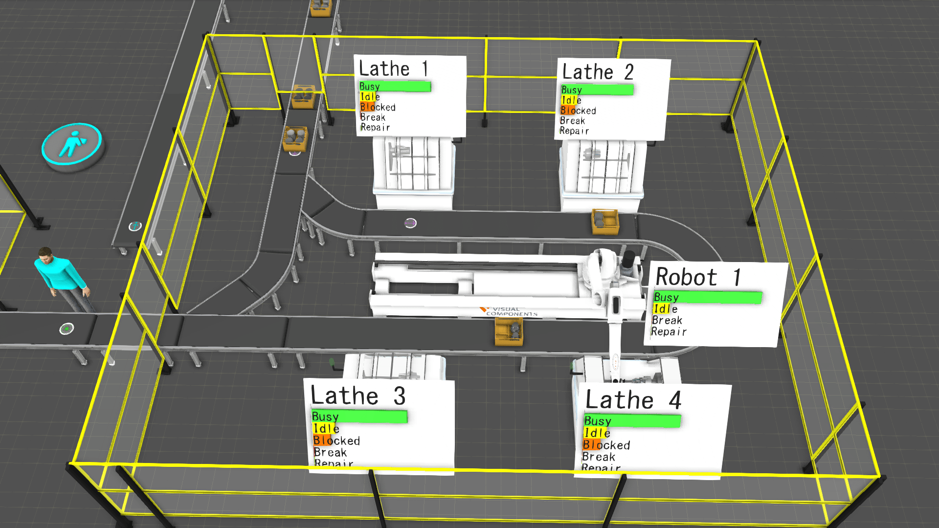
The top conveyor is used to feed out crates with faulty products that were detected by the quality checkpoint employee. After raw materials come into the system they are being processed by lathes. The layout with four lathes and a robot on a track has previously been evaluated as the best configuration for this scenario. Statistic panels on top of the lathes show their utilization.

Modelling quality inspection and quality-dependent conveyor routing

When all four cylinders of a crate have been processed they undergo quality inspection by a dedicated employee. The QA worker is one of a few human resources in this almost fully automated system. If a crate contains cylinders that do not meet the quality requirements, it is transported out of the system by the corresponding conveyor. Approved crates proceed to the palletizing station. The palletizing station has two pallet slots to ensure a continous flow while one of the pallets might be moved by an AGV.

Simulating AGV transport from final palletizing station in Visual Components

Once a pallet is full it is automatically transported to the high-bay storage by an AGV. In fact, the high-bay storage is an automatic storage and retrieval system (abbreviation: ASRS). The AGVs also ensure that pallet stations are supplied with new pallets. To ensure their continuous operation they also recharge automatically at a dedicated charging station. This charging station is located next to the pallet infeed.

High-bay storage and stacker crane simulation in Visual Components

High-bay storages are operated by an automatized stacker crane system. Pallets are distributed by product type and stored in a logical order. Once an order comes in for one or multiple pallets, the carriers automatically feed those pallets out to the conveyor on the right. Those pallets will then be moved to a truck loading area for final shipping.

Concluding remarks

The financial impact is one of the most important aspects to take into consideration when planning a new system. Simulating the development of financial KPIs does not only give an insight into how finances will perform over time. Moreover, such a simulation protects companies from initiating bad investments and incurring costs that could have been avoided. The result of a financial simulation supports the management’s decision with realistic and transparent facts regarding their potential investment.

In this article I used Visual Components as a simulation model development environment. But, there are many simulation tools available, each with their specific focus. For example, AnyLogic and simmer in R have also been introduced on this blog.

Johnny Camenzind

Founder and simulation developer at ProLean GmbH in Switzerland.
Over 6 years of experience with factory planning and process simulations.